Understanding Stochastic Differential Equations in the Context of Financial Markets

Financial markets are driven by unpredictable forces such as economic indicators, investor behavior, and geopolitical events. To model such randomness mathematically, Stochastic Differential Equations (SDEs) provide a powerful framework. SDEs extend ordinary differential equations by incorporating terms that model random noise, capturing the inherent uncertainty in asset price movements, interest rates, and volatility.

This article explains the fundamentals of stochastic differential equations, their mathematical formulation, and their crucial role in financial market modeling, pricing, and risk management.

Table of Contents

1. What Are Stochastic Differential Equations?

2. The Need for SDEs in Financial Modeling

3. Basic Components of SDEs

4. Brownian Motion and Wiener Processes

5. Itô Calculus: The Mathematics of SDEs

6. The Itô Integral and Itô’s Lemma

7. Common Financial Models Using SDEs

8. Geometric Brownian Motion (GBM) for Asset Prices

9. The Black-Scholes Model Derived from SDEs

10. Stochastic Volatility Models and SDEs

11. Interest Rate Models Using SDEs

12. Numerical Methods for Solving SDEs

13. Applications of SDEs in Risk Management

14. Limitations and Challenges

15. Conclusion

What Are Stochastic Differential Equations?

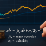
An SDE is a differential equation in which one or more terms are stochastic processes, meaning they have randomness. Formally, an SDE describes the evolution of a variable XtX_tXt​ over time with both deterministic and random components:

dXt=μ(Xt,t)dt+σ(Xt,t)dWtdX_t = \mu(X_t, t) dt + \sigma(X_t, t) dW_tdXt​=μ(Xt​,t)dt+σ(Xt​,t)dWt​

where:

• μ(Xt,t)\mu(X_t, t)μ(Xt​,t) is the drift term (deterministic trend)

• σ(Xt,t)\sigma(X_t, t)σ(Xt​,t) is the diffusion coefficient (volatility or noise intensity)

• dWtdW_tdWt​ is the increment of a Wiener process (Brownian motion)

The Need for SDEs in Financial Modeling

Financial variables such as stock prices and interest rates are continuous but subject to random fluctuations. Ordinary differential equations (ODEs) cannot capture this randomness. SDEs allow:

• Modeling of continuous-time stochastic processes

• Capturing random shocks and noise in asset dynamics

• Deriving pricing formulas for derivatives

• Simulating realistic market scenarios

Basic Components of SDEs

• Drift ($\mu$): The average or expected change rate of the process.

• Diffusion ($\sigma$): The volatility or randomness scale.

• Stochastic term: Modeled by increments of Brownian motion dWtdW_tdWt​, representing random shocks.

Brownian Motion and Wiener Processes

The Wiener process WtW_tWt​ is a continuous-time stochastic process with independent, normally distributed increments. It is the mathematical idealization of Brownian motion and serves as the fundamental source of randomness in SDEs.

Itô Calculus: The Mathematics of SDEs

Classical calculus does not apply to SDEs because Brownian paths are nowhere differentiable. Itô calculus provides tools for integration and differentiation when stochastic terms are involved.

The Itô Integral and Itô’s Lemma

• The Itô integral defines integration with respect to Brownian motion.

• Itô’s lemma is a stochastic version of the chain rule, used to find the differential of functions of stochastic processes.

Common Financial Models Using SDEs

• Geometric Brownian Motion (GBM): Models stock prices.

• Vasicek and CIR models: Model interest rates.

• Heston model: Models stochastic volatility.

Geometric Brownian Motion (GBM) for Asset Prices

GBM describes asset price StS_tSt​ evolution as:

dSt=μStdt+σStdWtdS_t = \mu S_t dt + \sigma S_t dW_tdSt​=μSt​dt+σSt​dWt​

Its solution models log-normal price distributions, foundational in option pricing.

The Black-Scholes Model Derived from SDEs

The Black-Scholes partial differential equation and option pricing formula are derived using SDEs describing underlying asset prices with GBM.

 Stochastic Volatility Models and SDEs

Models like Heston incorporate additional SDEs for volatility, capturing changing market uncertainty.

Interest Rate Models Using SDEs

Short rate models such as Vasicek and Cox-Ingersoll-Ross (CIR) use SDEs to describe random evolution of interest rates.

Numerical Methods for Solving SDEs

Analytical solutions are rare; numerical methods include:

• Euler-Maruyama scheme

• Milstein method

• Monte Carlo simulation

Applications of SDEs in Risk Management

SDEs help quantify risk measures, simulate scenarios, and perform stress testing.

 Limitations and Challenges

• Model assumptions may oversimplify reality.

• Parameter estimation is complex.

• Computational costs for high-dimensional systems.

Stochastic differential equations provide the mathematical backbone for modeling uncertainty in financial markets. Their ability to capture both deterministic trends and random fluctuations enables more accurate pricing, hedging, and risk assessment in complex financial environments.